A Plate Boundary Observatory
Paul G. Silver1, Yehuda Bock2, Duncan C. Agnew2,
Tom Henyey3, Alan T. Linde1 , Thomas V. McEvilly4
, Jean-Bernard Minster2, Barbara A. Romanowicz4 , I. Selwyn
Sacks1, Robert B. Smith5, Sean C. Solomon1
, Seth A. Stein6
1Carnegie Institution of Washington, DTM; 2IGPP,
Scripps Institution of Oceanography; 3University of Southern California/Southern
California Earthquake Center; 4University of California, Berkeley;
5University of Utah; 6Northwestern University/UNAVCO
 Figure
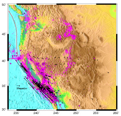
1. A topographic map of the western U.S., where the Pacific/North American plate
boundary zone reaches its greatest width. Also shown are the locations of earthquakes
above magnitude 6 that have occurred over the last 200 years (violet circles),
and background seismicity over the last 10 years (violet dots). This particular
plate boundary is very broad, containing about a third of the width of North
America, although the seismic activity is concentrated towards the western edge
of the boundary zone. Black arrows give GPS displacement vectors with respect
to stable North America for most available GPS data (Bennett et al., 1998).
Note large displacements along the San Andreas fault system and smaller, more
diffuse deformation in the Basin and Range. Red lines denote plate boundaries.
Figure
1. A topographic map of the western U.S., where the Pacific/North American plate
boundary zone reaches its greatest width. Also shown are the locations of earthquakes
above magnitude 6 that have occurred over the last 200 years (violet circles),
and background seismicity over the last 10 years (violet dots). This particular
plate boundary is very broad, containing about a third of the width of North
America, although the seismic activity is concentrated towards the western edge
of the boundary zone. Black arrows give GPS displacement vectors with respect
to stable North America for most available GPS data (Bennett et al., 1998).
Note large displacements along the San Andreas fault system and smaller, more
diffuse deformation in the Basin and Range. Red lines denote plate boundaries.
A basic tenet of plate tectonics is that plates are rigid and that deformation
is concentrated in narrow zones at their boundaries. We now know that plate
boundary deformation zones can actually be quite broad, often extending thousands
of kilometers into continental interiors, as illustrated by the Alpine-Himalayan
chain and the western cordilleras of North and South America. They account for
fully 15% of the Earth's surface (Gordon and Stein, 1992). Nearly all present-day
tectonic activity and most non-meteorological natural hazards, particularly
earthquakes and volcanic eruptions, are concentrated within these zones, making
the plate boundary zone a critical area of study both from scientific and societal
points of view. The segment of the Pacific-North American plate boundary zone
found in the western United States shares these characteristics. It covers a
third of the North American continent and includes such diverse features as
the Rocky Mountains, the Basin and Range, the Coast Ranges and the Sierras.
It also contains the seismogenic San Andreas fault system along its western
edge.
The diverse tectonic processes found in these zones are ultimately due to the
inexorable and quasi-steady relative motion of tectonic plates. An important
constraint provided by modern geodesy is that spatially averaged decadal geodetic
estimates of plate motion are, to first order, indistinguishable from geologic
estimates based on million-year time scales. This "steadiness" provides
a valuable framework for studying plate boundary deformation; it is also in
marked contrast to the extremely variable tectonic response to this motion.
This deformation spans at least 14 temporal and 3 to 5 spatial orders of magnitude,
and includes processes that range from mountain building to earthquake occurrence.
The study of plate boundary deformation is a rich research area that deserves
increased attention from a broad spectrum of Earth scientists. There are several
first-order unanswered questions that are nevertheless critical to understanding
any tectonic process.
- How is deformation accommodated three-dimensionally within a plate boundary
zone? On which time scales is it homogeneous and on which is it highly heterogeneous?
- What physically controls the spatial characteristics of plate boundary
deformation: the structural properties of the deformation zone, the characteristics
of the stress field, or an interaction of these factors?
- Are temporal variations in deformation controlled primarily by the slip-rate
on faults or the viscoelastic relaxation of the medium as a whole?
- Are there deformation transients, and do they propagate within the plate
boundary zone?
- What is the relation between vertical and horizontal tectonics? Is deformation
controlled primarily by direct interaction between the two plates, or does
the underlying mantle play a critical role?
- Of fundamental importance to seismology, how does plate motion ultimately
produce an earthquake? How do faults interact? How do earthquakes interact?
What fraction of fault slip is aseismic? What kinds of earthquake-related
transients are there? Do pre-event transients exist that may be utilized for
forecasting?
The central observational requirement for the study of plate boundary deformation
is the characterization of the three-dimensional deformation field over the
maximum ranges of spatial and temporal scales. The surface field can be measured
geodetically; instrumentation must provide: (i) sufficient coverage of the plate
boundary zone so as to capture an integral tectonic system, (ii) sufficient
station density for detecting localized (e. g., fault-specific) phenomena, and
(iii) the necessary bandwidth to detect plausible transient phenomena from fast
and slow earthquakes to strain buildup and viscoelastic relaxation. For studying
long-term, large scale tectonic processes, it is probably sufficient to examine
spatial variations in steady-state strain rate, which may then be compared to
geologically inferred deformation rates over the last few million years (Figure
1).
 Figure
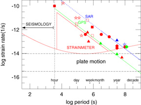
2. The necessary components of an integrated plate boundary deformation network,
and observed transients. Thresholds of strain-rate sensitivity (schematic) are
shown for strainmeters, GPS, and INSAR as functions of period. The diagonal
lines give GPS (green) and INSAR (blue) detection thresholds for 10-km baselines,
assuming 2-mm and 2-cm displacement resolution for GPS and INSAR, respectively
(horizontal only). GPS and INSAR strain-rate sensitivity is better at increasing
periods, allowing, for example, the detection of plate motion (dashed lines)
and long-term transients (periods greater than a month). Strainmeter detection
threshold (red) reaches a minimum at a period of a week and then increases at
longer period due to an increase in hydrologic influences. This is a conservative
estimate which has been bettered in some situations. At long periods (months
to a decade), GPS has greater sensitivity than strainmeters by one to two orders
of magnitude. At intermediate periods (weeks to months), sensitivities are comparable,
and at short periods (seconds to a month), strainmeter sensitivity is one to
three orders of magnitude greater than for GPS. Combined use of both data sets
provides enhanced sensitivity for detection of transients from earthquakes to
plate motion. Also shown are several types of transients observed by strainmeters
(red), GPS and equivalent (green), and INSAR (blue): Post-seismic deformation
(triangles), slow earthquakes (squares), long-term aseismic deformation (diamonds),
preseismic transients (circles), and volcanic strain transients (stars).
Figure
2. The necessary components of an integrated plate boundary deformation network,
and observed transients. Thresholds of strain-rate sensitivity (schematic) are
shown for strainmeters, GPS, and INSAR as functions of period. The diagonal
lines give GPS (green) and INSAR (blue) detection thresholds for 10-km baselines,
assuming 2-mm and 2-cm displacement resolution for GPS and INSAR, respectively
(horizontal only). GPS and INSAR strain-rate sensitivity is better at increasing
periods, allowing, for example, the detection of plate motion (dashed lines)
and long-term transients (periods greater than a month). Strainmeter detection
threshold (red) reaches a minimum at a period of a week and then increases at
longer period due to an increase in hydrologic influences. This is a conservative
estimate which has been bettered in some situations. At long periods (months
to a decade), GPS has greater sensitivity than strainmeters by one to two orders
of magnitude. At intermediate periods (weeks to months), sensitivities are comparable,
and at short periods (seconds to a month), strainmeter sensitivity is one to
three orders of magnitude greater than for GPS. Combined use of both data sets
provides enhanced sensitivity for detection of transients from earthquakes to
plate motion. Also shown are several types of transients observed by strainmeters
(red), GPS and equivalent (green), and INSAR (blue): Post-seismic deformation
(triangles), slow earthquakes (squares), long-term aseismic deformation (diamonds),
preseismic transients (circles), and volcanic strain transients (stars).
For short-term processes and their related deformation, such as earthquakes
and volcanic eruptions, temporal and spatial resolution becomes much more important.
Good sensitivity is needed across the sub-second-to-decade period band. The
sub-second to hour range is readily covered by seismological observations. At
longer periods, geodetic techniques are needed, but presently, there is no one
geodetic technique that spans this broad temporal range (5 orders of magnitude)
with roughly uniform strain-rate sensitivity. It will thus be necessary to utilize
several techniques, including strainmeters, GPS, and interferometric synthetic
aperture radar (INSAR) Ñthe first being most useful from an hour to a month
and the latter two (including non-continuous campaign measurements) for periods
longer than a month (Figure 2). The published observations of transient phenomena
reveal a variety of temporal scales that span this entire range (Figure 2).
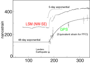
The post-seismic deformation of the 1992 Landers earthquake provides an excellent
example (Figure 3a). Transients with three distinct time constants have been
detected by these three instrumentation types: 5 days by strainmeters (Wyatt
et al., 1994), 48 days by GPS (Shen et al., 1994) and 3 years by INSAR (Massonnet
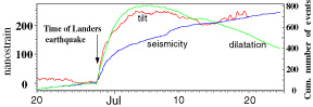
et al., 1996). In addition, remotely triggered seismicity from the Landers event
at Long Valley was accompanied by a 6-day deformation pulse observed clearly
on two strainmeters (Figure 3b, see Linde et al., 1994). These diverse post-seismic
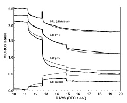
transients are suggestive of multiple deformation mechanisms. Two other examples
illustrate the potentially broad range of transient behavior. The first is a
slow earthquake (duration ~10 days) on the San Andreas fault near San Juan Bautista
that was detected on two strainmeters, and was accompanied by increased seismic
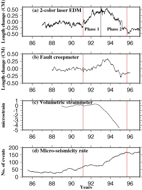
activity (Figure 3c, Linde et al., 1996). The other is a long-term (multi-year)
aseismic transient in San Andreas fault slip that was observed on 2-color geodimeters,
strainmeters, and creepmeters, and was coincident with an increase in seismicity
(Figure 3d, Gao et al., 1998). Clearly, a crucial task in utilizing a multicomponent
system is the integration of these geodetic techniques. There are ongoing efforts
by investigators to incorporate at least two of these techniques into an internally
consistent measure of the surface strain field: GPS and INSAR (Bock and Williams,
1997), and GPS and strainmeters (Gao et al., 1998).
Figure 3: Examples of transients: a) Post-seismic deformation for the
1992 Landers earthquake from a laser strainmeter (LSM) and GPS, illustrating
5-day and 48-day time constants, respectively (after Wyatt et al., 1994). (b)
Landers-triggered strain transient produced at Long Valley. Produced increase
in seismicity (blue) and observed by a dilatometer (green) and tiltmeter(green)
20km apart (After Linde et al, 1994). (c) Slow (10-day) earthquake detected
along the San Andreas fault at San Juan Bautista (south of Bay Area) and accompanied
by elevated seismicity (Linde et al., 1996). (d) Multiyear aseismic transient
in San Andreas fault slip at Parkfield, observed on 2-color geodimeters (stack
of fault-crossing lines, GPS equivalent), dilatometers and tensor strain (not
shown), creepmeters, and accompanying increased seismicity. The increase and
decrease in line length (top panel) between 1991-1993 and 1993-1996 corresponds
to a decrease and increase in fault slip rate, respectively (Gao et al.,1998).
Determining strain at depth is a less straightforward but crucial task. Deformation
within the seismogenic zone, for example, may provide vital information on the
triggering of seismic events. Strain indicators rather than calibrated strainmeters,
must be used, however. For example, microearthquake activity can be interpreted
as the radiated component of deformation in the seismogenic zone. Recent results
of cluster analysis of microearthquakes at Parkfield have demonstrated the power
of this type of technique for furthering our understanding of fault zone processes
(Nadeau et al., 1995). Another important approach is imaging spatial and temporal
variability in crustal structure. Images of faults can be obtained by the use
of fault-zone guided waves (e.g., Li et al., 1997). The seismological detection
of strain-induced opening and closing of fluid-filled cracks can be achieved
through characterizing temporal variations in crustal structure. Mantle deformation
is also accessible by seismic imaging, through constraints on the thermal (tomography)
and strain (anisotropy) fields.
 Figure
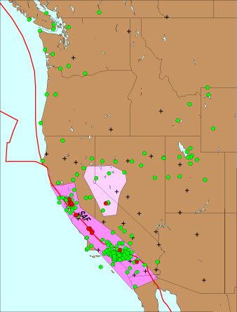
4. Existing and planned GPS (green circles), strainmeter installations (red
circles), and three-component broadband seismographs (crosses). Pink zones denote
most seismogenic part of the plate boundary (see Figure 1). These zones, shaded
dark and light pink, correspond to areas of high and low population density,
respectively. The PBO would be concentrated in these areas, factoring in population
density in deployment priorities. The rest of the plate boundary (brown) would
have more sparsely distributed instrumentation.
Figure
4. Existing and planned GPS (green circles), strainmeter installations (red
circles), and three-component broadband seismographs (crosses). Pink zones denote
most seismogenic part of the plate boundary (see Figure 1). These zones, shaded
dark and light pink, correspond to areas of high and low population density,
respectively. The PBO would be concentrated in these areas, factoring in population
density in deployment priorities. The rest of the plate boundary (brown) would
have more sparsely distributed instrumentation.
With these issues in mind, we recommend that the scientific community consider
establishing a strain observatory along the Pacific/North American plate boundary
(hereafter referred to as the Plate Boundary Observatory or PBO). The PBO should
measure deformation over a broad spectrum of spatial and temporal scales and
provide sufficient spatio-temporal resolution to constrain any transients associated
with short-wavelength phenomena such as earthquakes. We propose that, where
such phenomena are most prevalent, namely the most seismogenic areas of the
boundary, 10-km spacing of instruments be achieved (Figure 4). This portion
of the plate boundary is also where the greatest temporal resolution is needed.
A close integration of seismometers, strainmeters, GPS, and INSAR is necessary
to provide uniform strain-rate sensitivity, at plate-motion strain rates, across
the temporal band from several Hertz to a decade. On the order of 1000 observing
sites would be required. For the broader plate boundary, it would be possible
to use coarser spacing, and to utilize GPS and INSAR exclusively, since these
techniques are most successful for detecting long-period or steady-state strain.
Constraints on the subsurface deformation field would be supplied by studies
of strain indicators: microeathquake activity and crustal and mantle structure
(including possible temporal variations). The seismological component would
require both an augmentation of permanent seismic instrumentation in the plate
boundary zone and transportable array deployments to map out particular regions
in detail.
It would not be necessary to start from scratch in this effort, since some
pieces of the PBO are already, or will soon be, in place (Figure 4). The most
advanced component consists of geodetic-quality arrays of continuous GPS stations
in southern (SCIGN) and northern (BARD) California, northern (NBAR) and eastern
(EBAR) Basin and Range, and the Pacific Northwest (PANGA) (Figure 4). There
are presently about 200 GPS receivers deployed in the proposed area, and 250
more should be installed within the next 1 to 2 years. The strainmeter component
is much less advanced, since there are only about 20 strainmeter sites along
the entire San Andreas fault system. Regarding INSAR, images are being acquired
by non-U.S. satellites over western North America and are available to U.S.
investigators, although issues of data access remain.
The establishment of a fully capable plate boundary observatory will require
progress in four areas: (i) A more effective integration of strainmeters and
GPS for a truly broadband plate boundary observatory. This integration concept
should first be tested on a smaller scale, limited to a region of the plate
boundary, where there are GPS receivers and strainmeters in roughly equal numbers.
(ii) The densification of geodetic and seismic instrumentation along the northern
San Andreas fault system for increased spatial resolution. (iii) The linking
of the northern and southern San Andreas zones, to cover the seismogenic part
of the plate boundary. (iv) Improving access to INSAR data for more effective
integration. Present efforts involve operating a downlink facility in cooperation
with the European Space Agency, and/or launching a SAR satellite that would
collect data over western North America on a regular basis.
While the main focus of the PBO would be to gain a basic understanding of plate
boundary processes, the PBO would also provide information of immense practical
value. In particular, we would be in a position to detect precursory strain
transients that may prove practical for the forecasting of earthquakes and volcanic
eruptions. Such precursors exist for volcanic eruptions and have already been
used to make predictions. Whether such precursors exist for earthquakes as well
is something we still have to find out. The answer to this question would be
crucial knowledge for society.
References
Bennett, R.A., J.L. Davis, B.P. Wernicke, The present-day pattern of western
U.S. Cordillera deformation, Geology, 1998, submitted.
Bock, Y., and S. Williams, Integrated satellite interferometry in southern
California, EOS Trans. AGU, 78, pp. 293, 299-300, 1997.
Gao, S., P. G. Silver, and A. T. Linde, A comprehensive analysis of deformation
data at Parkfield, California: Detection of a long-term strain transient,
J. Geophys. Res., submitted, 1998.
Gordon, R. G. and S. Stein, Global tectonics and space geodesy, Science,
256, 333-342, 1992.
Li, Y. G., K. Aki and F. L. Vernon, San Jacinto fault zone guided waves;
a discrimination for recently active fault strands near Anza, California,
J. Geophys. Res., 102, 11,689-11,701, 1997
Linde, A. T. I. S. Sacks, M. Johnston, D. Hill and R. Bilham, Increased pressure
from rising bubbles as a mechanism for remotely triggered seismicity, Nature,
371, 408-410.
Linde, A. T., M. T. Gladwin, M. J. S. Johnston, R. L. Gwyther, and R. G.
Bilham, A slow earthquake sequence on the San Andreas fault, Nature, 383,
65-68, 1996.
Massonnet, D., W. Thatcher, and H. Vadon, Detection of postseismic fault-zone
collapse following the Landers earthquake, Nature, 382, 612-616, 1996.
Nadeau, R. M., W. Foxall, and T. V. McEvilly, Clustering and periodic recurrence
of microearthquakes on the San Andreas Fault at Parkfield, California, Science,
267, 503-507, 1995.
Shen, Z., D. D. Jackson, Y. Feng, M. Cline, M. Kim, P. Fang, and Y. Bock,
Postseismic deformation following the Landers earthquake, California, 28 June
1992, Bull. Seismol. Soc. Am. 84, 780-791, 1994.
Wyatt, F. K., D. C. Agnew, and M. Gladwin, Continuous measurements of crustal
deformation for the 1992 Landers earthquake sequence, Bull. Seismol. Soc.
Am., 84, 646-659, 1994.
Return to: IRIS Newsletter
Information
Return to: Title Page and Table of Contents
Continue to: Next Article